Off on a Tangent

The sun is shining, and the breeze entices the leaves of your grand apple tree to sing a joyous tune. You sit at the edge of the balcony and watch the tree branches dance to the rhythm of their song. Amidst the poetry, an apple is fed up with the palpable pretentiousness, and detaches himself from the scene, awaiting the soothing embrace of the grass blades beneath.

As the apple of your eye descends to the earth, you wonder… how fast did the apple fall after one second?

At first, this question seems entirely reasonable… until you realise it doesn’t really make sense. The speed of a car, for instance, is usually measured in kilometres per hour (that is, assuming you live in a country that uses metric), which tells you how many kilometres your vehicle would cover if you maintained the given speed for exactly one hour. In order to determine the (average) velocity of an object—such as a car, or your dear apple—you need to calculate

$\displaystyle \mathrm{velocity} = \frac{\text{change in position}}{\text{change in time}}$

In fancier (i.e., mathematical and physical) notation, this would be written as

$\displaystyle v = \frac{\Delta x}{\Delta t}$

In particular, the calculation of velocity requires sampling at two separate times. Therefore, it’s rather nonsensical to ask for how quickly an apple is moving at a single specific time; that’s like taking a snapshot of the falling apple and trying to use this to determine its velocity.

This doesn’t deter you, though, since there still seems to be some merit behind the concept of an “instantaneous velocity.” So, you try to approximate what this quantity should be. You try sampling the position of the apple every $\Delta t=0.5$ seconds and plot the result:

To estimate the instantaneous velocity at time $t=1$ (i.e., at the red dot), you consider the average velocity for the 0.5 seconds before the red dot, and also the average velocity for the 0.5 seconds after the red dot:

These tell you that what would be the instantaneous velocity must have been somewhere near 7.3 and 12.3 metres per second. To improve the approximation, you sample more frequently, thus making $\Delta t$ smaller and smaller.

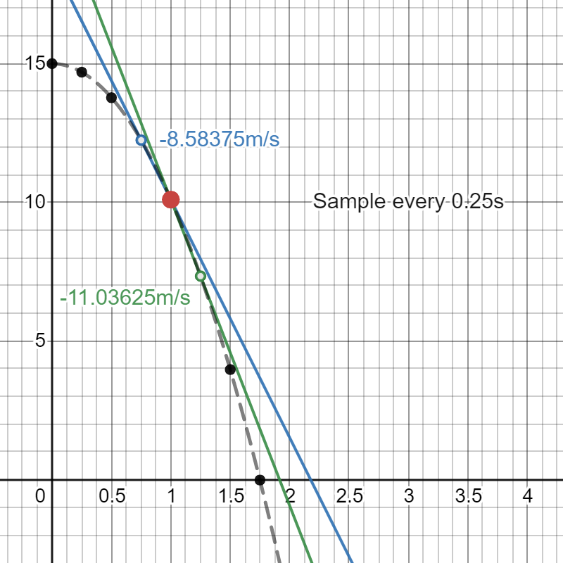
(You can experiment with this yourself on Desmos.) As $\Delta t$ decreases, you notice that the blue and green lines start to stabilise, and with further investigating, the numbers seem to be converging to about 9.81 metres per second. Therefore, you declare that the apple fell at around 9.81 metres per second exactly one second after falling off the tree. This makes a lot of sense, so you declare this to be your definition of instantaneous velocity.

More precisely: if the position (say, of your apple) is given as a function $x(t)$ of time, then the instantaneous velocity at a specific time is given to be the number that the average speed $\frac{\Delta x}{\Delta t}$ gets really close to when you take $\Delta t$ to be smaller and smaller. Since $\Delta$ is the Greek letter D and represents “change,” you might think it cute to denote “really small change” by a little $\mathrm d$ : that is, if $\Delta x$ represents a “change in position,” then $\mathrm dx$ should represent a “really small change in position.”

In mathematical language, the value $\frac{\Delta x}{\Delta t}$ approaches when you take $\Delta t$ to be smaller and smaller is called the limit of $\frac{\Delta x}{\Delta t}$ as $\Delta t\to0$ . Think of the limit as a constraint on $\frac{\Delta x}{\Delta t}$ , forcing $\frac{\Delta x}{\Delta t}$ to be really close to the limit when $\Delta t$ is really close to zero. To summarise, your instantaneous velocity takes the symbolic equation

$\displaystyle v = \frac{\mathrm dx}{\mathrm dt} = \lim_{\Delta t\to0}\frac{\Delta x}{\Delta t}$

The derivative

Moving away from physics, you realise that you can do the same thing with other functions $y=f(x)$ . The simplest functions are given by lines, which can be defined by the equation $y = mx + b$ . Here, $b$ tells us where the line crosses the $y$ -axis, but the more important parameter is $m$ , which is called the slope of the line. Explicitly, the slope describes how quickly $y$ changes based on how much $x$ changes, which can be stated as

$\displaystyle m = \frac{\Delta y}{\Delta x} = \frac{\text{change in }y}{\text{change in }x}$

With the ideas behind instantaneous velocities, you realise that you can begin to make sense of instantaneous slopes of a function: if you have a function $f(x)$ , then you can define its instantaneous slope at a specified point to be

$\displaystyle \frac{\mathrm df}{\mathrm dx} = \lim_{\Delta x\to0}\frac{\Delta f}{\Delta x} = \lim_{\Delta x\to0}\frac{f(x+\Delta x)-f(x)}{\Delta x}$

The instantaneous slope at a point $x$ is more precisely called the derivative of $f(x)$ at the point $x$ . Therefore, you can use this terminology to say that “velocity is the derivative of position with respect to time.”

However, you quickly realise that not all functions have derivatives. For example, the absolute value function

does not have a well-defined derivative at zero (sampling right before zero gives you a slope of $-1$ while sampling right after zero gives you a slope of $1$ ; no matter how close together your samples are, they never approach any limit—in other words, the derivative does not exist). You observe that the cause of this problem is the sharp corner at zero: the derivative of a function only exists if the function looks sufficiently “smooth,” meaning that the function should already look like a line if you zoom in closely enough. Such functions are called differentiable: this is because computing the derivative is called “differentiation” (it computes the ratio between the difference of outputs and the difference of inputs).

In other words, if you look closely enough at the point $x_0$ , a differentiable function $f(x)$ should look something like $y=mx+b$ for an appropriate line. The slope of this approximate line is exactly the derivative: $m=\frac{\mathrm df}{\mathrm dx}$ .

What this means more concretely is that when you’re close to a point $x_0$ , then $f(x)$ looks approximately like the line

$\displaystyle y = f(x_0) + \frac{\mathrm df}{\mathrm dx}(x_0)\cdot(x-x_0)$

which is then called the linear approximation of $f(x)$ near $x_0$ . In mathematical symbols, this reads as

$\displaystyle \Delta f =\frac{\mathrm df}{\mathrm dx}(x_0)\cdot\Delta x + o(\Delta x)$

where $o(\Delta x)$ denotes a quantity that is significantly smaller than $\Delta x$ as $\Delta x\to0$ .

Note. If the change in $x$ is small enough (so that $o(\mathrm dx) = 0$ ), the above identity becomes $\mathrm df = \frac{\mathrm df}{\mathrm dx}\cdot\mathrm dx$ , which looks like an “obvious” identity, but is the more precise definition of the differential of $f$ .

If you were to graph the linear approximation of a function (e.g., for the position of a falling apple), you get a better idea what this line really is:

For a sufficiently smooth function, the linear approximation gives us the line that lies tangent to our function at the point; that is, the line that seems to just “touch” our function without blatantly impaling it. By looking at the graph, you can also see that the linear approximation is actually quite good at estimating differentiable functions! This has great consequences for simplifying calculation and analysis:

$\displaystyle y = \frac{\sin x\cos x+e^x}{x^2+x+1}$ is basically the same as $y = x+1$ when $x$ is very small^{[see for yourself]}.

The concept of tangents (like the above) is a way of formalising “flattening” shapes while retaining as much information as possible. This is the idea underlying why you can use a flat, two-dimensional map of a city and reliably eyeball how distances, angles, and sizes compare between different locations, despite the general spherical shape of the Earth: a city is so small compared to the whole Earth that a map—which is exactly a (scaled-down) linear approximation of the true city—barely differs in geometry from the city itself.

For the record, the same cannot be said about any flat, two-dimensional map of the western hemisphere, by the Theorema Egregium.

This being said, we haven’t yet established the mathematics necessary to talk about tangent planes of the Earth. As a first step, we would need to establish a theory of higher-dimensional differentiable functions.

The derivative, in many variables

For example, let’s consider a function $f:\mathbb{R}^2\to\mathbb{R}$ . This means that our function takes two inputs $x,y$ and produces a single output $f(x,y)$ . What should the “derivative” of such a function be? In the one-dimensional case, the derivative was just a number, and this number represented the slope of the tangent line, so a good start is to expect that the derivative of our $f(x,y)$ ought to measure the “slope” of a tangent plane.

Therefore, declare $f(x,y)$ to be differentiable at a point $(x_0,y_0)$ if near this point, the function looks approximately like a plane in 3D space

$z = Ax + By + C$

Based off of the same discussion in the one-dimensional case, it’s natural to expect that the “derivative” of $f(x,y)$ should encode the coefficients $A$ and $B$ . In particular, the “derivative” should no longer be a single number, but rather a two-dimensional vector.

Understanding one-dimensional derivatives turns out to be sufficient for determining what the coefficients $A$ and $B$ should be. To illustrate, let’s determine $A$ . The trick is to think of $x$ as an input variable, and think of $y=y_0$ as a fixed constant, so that $f(x,y_0)$ is a one-variable function. Then, our “planar approximation” $z=Ax + By + C$ reduces to a linear approximation

$z = \underbrace{Ax}_{mx} + \underbrace{By_0 + C}_b$

for the function $f(-,y_0)$ . Therefore, the coefficient $A$ —being the slope of this linear approximation—must be the derivative of $f(x,y_0)$ with respect to $x$ . Since this computes part of the derivative for the two-variable function $f$ , we call this the partial derivative of $f(x,y)$ with respect to $x$ :

$\displaystyle \frac{\partial f}{\partial x}(x_0,y_0) = \frac{\mathrm df(-,y_0)}{\mathrm dx}(x_0) = \lim_{\Delta x\to0}\frac{f(x_0+\Delta x,y_0)-f(x_0,y_0)}{\Delta x}$

Entirely analogously, the coefficient $B$ is the partial derivative of $f(x_0,y)$ with respect to $y$ :

$\displaystyle \frac{\partial f}{\partial y}(x_0,y_0) = \frac{\mathrm df(x_0,-)}{\mathrm dy}(y_0) = \lim_{\Delta y\to0}\frac{f(x_0,y_0+\Delta y)-f(x_0,y_0)}{\Delta y}$

In summary, a two-dimensional differentiable function admits a planar approximation (which is actually still just called a linear approximation) of the form

$\displaystyle \Delta f = \frac{\partial f}{\partial x}(x_0,y_0)\cdot\Delta x + \frac{\partial f}{\partial y}(x_0,y_0)\cdot\Delta y + o(\Delta x,\Delta y)$

Note. By taking the changes in $x$ and $y$ to be very small again, you obtain the definition of the differential of a two-dimensional function $f$ , which is $\mathrm df = \frac{\partial f}{\partial x }\mathrm dx + \frac{\partial f}{\partial y}\mathrm dy$ .

The two-dimensional vector which collects these partial derivatives is called the gradient of $f$ and denoted $\nabla f = \begin{bmatrix} \frac{\partial f}{\partial x} & \frac{\partial f}{\partial y} \end{bmatrix}$ , and this serves as the “derivative” of $f(x,y)$ .

The story is exactly the same for higher-dimensional functions $f:\mathbb R^n\to\mathbb R$ . Write $\vec x = (x_1,\dots,x_n)$ for the vector of inputs to our function, so that $f(\vec x)=f(x_1,\dots,x_n)$ . If $f(\vec x)$ is differentiable, then we can compute its partial derivatives $\frac{\partial f}{\partial x_i}$ for every $1\leq i\leq n$ , and these give us the linear approximation

$\displaystyle \Delta f = \frac{\partial f}{\partial x_1}(\vec x)\cdot\Delta x_1 + \frac{\partial f}{\partial x_2}(\vec x)\cdot\Delta x_2 + \dots + \frac{\partial f}{\partial x_n}(\vec x)\cdot\Delta x_n + o(\Delta\vec x)$

Using Sigma notation, this equation can be written more briefly as

$\displaystyle \Delta f = \sum_{i=1}^n\frac{\partial f}{\partial x_i}(\vec x)\cdot\Delta x_i + o(\Delta\vec x)$

and the gradient (“derivative”) of $f$ is the $n$ -dimensional vector

$\nabla f = \begin{bmatrix} \frac{\partial f}{\partial x_1} & \frac{\partial f}{\partial x_2} & \dots & \frac{\partial f}{\partial x_n} \end{bmatrix}$

It’s more useful to think of $\nabla f$ as a (row) vector rather than just a list of numbers. Indeed, one advantage is that it makes computing directional derivatives much easier. The partial derivative $\frac{\partial f}{\partial x_i}$ describes the rate of change of $f$ as you vary $x_i$ specifically: in other words, it is the slope of the line that lies tangent to the graph of $f$ and points in the direction of $x_i$ . Therefore, we can think of it as a directional derivative of $f$ in the direction $x_i$ . If you wanted to compute the derivative of $f$ in the direction of an arbitrary* vector $\vec v$ , the precise definition is the familiar-looking limit

$\displaystyle \nabla_{\vec v}f(\vec x) = \lim_{\Delta t\to0}\frac{f(\vec x + \Delta t\vec v) - f(\vec x)}{\Delta t}$

However, with the gradient vector of a differentiable function, you can compute the directional derivative more simply as the dot product $\nabla_{\vec v}f(\vec x) = \nabla f(\vec x)\cdot\vec v$ .

*Technical remark. The direction for a directional derivative should be a unit vector. However, if $\vec v$ is not a unit vector, then you can think of $\nabla_{\vec v}f$ as being the rate of change of $f$ when running with velocity $\vec v$ per unit time.

A related advantage of taking the gradient to be a (row) vector rather than just a list of numbers is that it allows us to rewrite the linear approximation of $f(\vec x)$ with the dot product as

$\displaystyle \Delta f = \nabla f(\vec x)\cdot\Delta\vec x + o(\Delta\vec x)$

showing how the multivariable story is very much the same as the one-dimensional story we started with.

Remark. I am aware of the unfortunate notation clash. When I write $\Delta f$ , I am definitely not referring to the Laplacian.

Moreover, this presentation of the linear approximation suggests that we shouldn’t think of the derivative of a function as a mere number, but rather as a linear transformation. This becomes particularly handy when you try to generalise the derivative further to handle a multivariable vector-valued function $f:\mathbb{R}^n\to\mathbb{R}^m$ . Now, the total derivative of the function $f$ at a point $\vec x$ is the unique linear operator $\mathrm Df_{\vec x} : \mathbb{R}^n\to\mathbb{R}^m$ such that

$\Delta f = \mathrm Df_{\vec x}(\Delta\vec x) + \vec o(\Delta\vec x)$

Equivalently (if you like to bring limits into the story), the total derivative is the unique operator such that

$\displaystyle \lim_{\Delta\vec x\to\vec 0}\frac{\left\|f(\vec x + \Delta\vec x) - f(\vec x) - \mathrm Df_{\vec x}(\Delta\vec x)\right\|}{\|\Delta\vec x\|} = 0$

Write $f = (f_1,\dots,f_m)$ as a (column) vector, then each $f_i:\mathbb{R}^n\to\mathbb{R}$ is a multivariable differentiable function. Therefore, we can apply our knowledge of gradients to determine what the total derivative of $f$ looks like row by row. Since $\mathrm Df$ is a linear operator, fix the standard bases for $\mathbb{R}^n$ and $\mathbb{R}^m$ , then $\mathrm Df$ admits an $m\times n$ matrix representation

$\displaystyle \mathrm Df = \begin{bmatrix} \nabla f_1 \\ \nabla f_2 \\ \vdots \\ \nabla f_m \end{bmatrix} = \begin{bmatrix} \frac{\partial f_1}{\partial x_1} & \frac{\partial f_1}{\partial x_2} & \dots & \frac{\partial f_1}{\partial x_n} \\ \frac{\partial f_2}{\partial x_1} & \frac{\partial f_2}{\partial x_2} & \dots & \frac{\partial f_2}{\partial x_n} \\ \vdots & \vdots & \ddots & \vdots \\ \frac{\partial f_m}{\partial x_1} & \frac{\partial f_m}{\partial x_2} & \dots & \frac{\partial f_m}{\partial x_n} \end{bmatrix}$

which is called the Jacobian of $f$ .

This more general theory of differential calculus is quite versatile, and allows us to compute tangents and linear approximations for many things. For instance, we can model the hills or mountains with a smooth function $M : \mathbb{R}^2\to\mathbb{R}$ , where $M(x,y)$ tells you what the elevation level is at coordinates $(x,y)$ , and differential calculus can tell us how steep these hills can get, where the peaks and troughs are, etc. For another example, we can model the trajectory of a particle with a smooth function $p:\mathbb R\to\mathbb{R}^3$ , where $p(t)=(p_x(t),p_y(t),p_z(t))$ describes the coordinates of the particle in 3D space at time $t$ , and differential calculus can tell us the velocity of the particle at any point in time.

However, we still haven’t quite developed enough mathematics to talk about the surface of the Earth. The issue with smooth geometric shapes—such as ellipses, spheres, tori (i.e., doughnuts), or any kind of blob existing in higher-dimensional space—is that they are typically not graphs of functions. For example, a unit circle centred at the origin has two $y$ -values for every $-1<x<1$ , so it’s more appropriately plotted as two functions: $y=\sqrt{1-x^2}$ (red) and $y=-\sqrt{1-x^2}$ (blue):

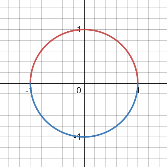
This almost seems to solve the issue: you can then use differential calculus on the two functions to compute tangent lines and the whole works. However, this isn’t perfect: even just on the circle presented above, we cannot use the function decomposition to compute the tangent lines where $x=1$ or $x=-1$ : neither function is actually differentiable at these points. What’s also an issue is that the tangent lines at these points are vertical, and thus cannot be described as functions of $x$ .

“The Earth isn’t flat, but it’s close”

The idea is so close to working, though, so the idea is to modify this kind of deconstruction so that it doesn’t depend on how we draw our geometric shape in Euclidean space ( $\mathbb{R}^n$ ). This leads to the idea of a smooth manifold. Loosely speaking, a smooth $n$ -dimensional manifold (also called a smooth $n$ -manifold) is a shape $M$ such that for every point $p\in M$ , there is a way to smoothly transform a region of $M$ close to $p$ into a subspace of $\mathbb{R}^n$ .

For example, consider the unit circle again: this should be a smooth 1-manifold, so consider the point at the north pole. The figure below shows how to smoothly transform the upper semicircle into a straight line:

Try sliding the orange intermediate line on Desmos

These smooth transformations allow you to define a local coordinate system on your manifold; that is, when you’re near a point $p$ of your $n$ -manifold, you can describe your position relative to $p$ with ordinary Euclidean coordinates $(x_1,\dots,x_n)$ . The fact that the surface of the Earth is a smooth 2-manifold is why a map of the city can be navigated using a compass (i.e., $x$ and $y$ coordinates).

Using the map analogy, you can equivalently describe a smooth $n$ -manifold as a space that can be covered with $n$ -dimensional “maps” of regions of the manifold, such that the “maps” agree where they overlap on the manifold. The local coordinate systems are then the coordinate systems of these “maps.” Appropriately, the collection of “maps” on a smooth $n$ -manifold is called an atlas.

Formal definition (skippable). A smooth $n$ -manifold is a Hausdorff and second-countable topological space $M$ equipped with a smooth atlas, which is an open cover $\{U_\alpha\}_{\alpha\in I}$ paired with a family of open embeddings $\varphi_\alpha : U \hookrightarrow \mathbb{R}^n$ called charts. These charts are required to be smoothly compatible in the sense that the transition maps $\varphi_\beta\varphi_\alpha^{-1} |: \varphi_\alpha(U_\alpha\cap U_\beta) \to \varphi_\beta(U_\alpha\cap U_\beta)$ are $C^\infty$ -functions (meaning they are infinitely differentiable: we can take arbitrarily high-order mixed partial derivatives).

Let $M,N$ be smooth manifolds (of possibly differing dimensions), with respective atlases $\{U_\alpha,\varphi_\alpha\}_{\alpha\in I}$ and $\{V_\beta,\psi_\beta\}_{\beta\in J}$ . A continuous function $f:M\to N$ is a smooth map of manifolds if the maps $\psi_\beta f\varphi_\alpha^{-1}$ are $C^\infty$ -functions where defined.

The atlas provides us with a local coordinate system: for a point $p\in M$ , we get coordinates $x_1,\dots,x_n$ through the embedding $\varphi_\alpha$ where $U_\alpha\ni p$ : more precisely, the coordinates of a nearby point $p'$ (i.e., $p'\in U_\alpha$ ) in this coordinate system is just the coordinates of the vector $\varphi_\alpha(p')-\varphi_\alpha(p)\in\mathbb{R}^n$ . If $f:M\to N$ is a map of smooth manifolds, then it induces $C^\infty$ functions on the local coordinates (which reduces its theory to the multivariable calculus described earlier).

Now, suppose we have a smooth function $f:M\to N$ of manifolds. If $\dim M=m$ and $\dim N=n$ , then at any point $p\in M$ we can find a local coordinate system $x_1,\dots,x_m$ around $p$ , and a local coordinate system $y_1,\dots,y_n$ around $f(p)\in N$ so that (locally) this smooth function looks like a smooth map $f:\mathbb{R}^m\to\mathbb{R}^n$ .

Therefore, we can reuse the theory already developed for derivatives of multivariable functions to compute the total derivative of $f$ at this point and get a linear operator $\mathrm Df_p:\mathbb{R}^m\to\mathbb{R}^n$ . Since derivatives are a local property, this should be the correct “derivative” of our smooth function of manifolds, but what does it mean?

Remember that we first interpreted the total derivative of an ordinary multivariable function at a point as the best linear approximation of the function at the chosen point. This made a lot of sense in Euclidean space $\mathbb{R}^n$ because this space is inherently “linear” itself. Now, we’re on a general manifold—there’s no natural “linear” structure on an entire sphere. But, maybe we can find linear structure locally: if we’re going to look at our function closely around a point, then we might as well do the same to our manifold.

The atlas on a manifold $M$ is enough to convince tiny conspiracy theorists living there that the world is flat, so zooming in this far, it almost looks like the manifold is a vector space! However, it’s not: a vector space goes off to infinity in every direction, but a local coordinate system is only good for a relatively small piece of our manifold. Consider the 2-manifold that we call Earth. With an atlas of the globe, we have local two-dimensional coordinates that we Earthlings typically refer to as the compass directions*. They’re “local” because they only make sense for a certain distance, after which the direction stops really making sense. For example: I can say that Saskatchewan is to the east of Alberta, and even that Québec is to the east of Alberta. However, if I “keep going east,” it becomes less apparent: is Germany to the east of Alberta? What if I go so far “east” that I wrap the Earth and end up in British Columba… does that make it east of Alberta?

*Technical remark. The compass directions don’t actually make sense at the north and south poles, but they work as local coordinates everywhere else. Just use it as a fairly robust analogy of what local coordinates are—you can’t define a smoothly varying local coordinate system on $2n$ -dimensional spheres thanks to the hairy ball theorem.

The problem is that the compass directions aren’t actually supposed to curve with the Earth: they should instead span a flat plane that shoots off the Earth from your reference point:

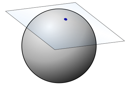
As you can see, what we really want is to look at the tangent spaces on our manifold! The local coordinates are not directly part of the tangent space since they are glued to the manifold itself and stop making sense if you move too far away from your starting point (because they’re local coordinates). How, then, do we escape the confines of our manifold?

The derivative of the Earth

Well, we do it by running. Imagine you’re running in a straight line on Earth, and then suddenly gravity “turns off.” What happens? You’ll start shooting off in the direction you were running (i.e., in the direction of your velocity vector): this direction sits tangent to the Earth! This is exactly how the tangent space on a manifold is defined: the tangent space at a point $p\in M$ is the space $T_pM$ of all possible velocity vectors that could be realised if you were to run on $M$ and step at the point $p$ .

What does this mean more mathematically? Let’s say $\gamma(t)$ describes where you are during your run on the manifold at time $t$ . For simplicity, let’s say you are at point $p$ at time $t=0$ (i.e., $\gamma(0) = p$ ). Using the local coordinates around $p$ , we are allowed to think of $\gamma$ as a smooth function $\gamma:\mathbb{R}\to\mathbb{R}^n$ .

Just as in the beginning of this story, velocity is given as the derivative of position with respect to time, so the instantaneous velocity vector for $\gamma$ at time $t=0$ is simply the $n$ -dimensional vector

$\displaystyle \left.\frac{\mathrm d\gamma}{\mathrm dt}\right|_{t=0} = \begin{bmatrix} \frac{\mathrm d\gamma_1}{\mathrm dt}(0) \\ \vdots \\ \frac{\mathrm d\gamma_n}{\mathrm dt}(0) \end{bmatrix}$

It follows that all tangent spaces of an $n$ -dimensional manifold are $n$ -dimensional vector spaces. In particular, consider paths $e_i(t)$ that run in the direction of the local coordinate $x_i$ for each $1\leq i\leq n$ . Their corresponding velocity vectors then form a basis of $T_pM$ .

Let’s apply this to the 2-manifold we call Earth. The tangent space is spanned by the velocity vectors $e_{\mathrm{North}}(t)$ and $e_{\mathrm{East}}(t)$ , so this recovers our original realisation of its tangent space discussed earlier.

This technically completes the story of finding tangents on a manifold, but this sort of definition of the tangent space is… clunky. First, if given a tangent vector, it’s difficult to recover a path whose instantaneous velocity is given by this vector. Secondly, this definition seems to depend on our choice of local coordinates. Not every manifold has a natural or obvious local coordinate system at every point, so it would be better if the tangent space could be defined independently of any choice of coordinates.

To find a better definition, we work backwards: let’s suppose $\vec v$ is a tangent vector of our manifold $M$ at a point $p\in M$ . While we may not know what path $\gamma$ obtains $\vec v$ as its velocity vector, but we do know that $\vec v$ describes a direction from the point $p$ . This enables us to talk about directional derivatives again! But this time, we are speaking of directional derivatives of smooth functions $f:M\to\mathbb{R}$ , at least locally around $p$ . Let’s denote this directional derivative by $D_{\vec v}f|_p$ .

If we think locally, a smooth function $f:M\to\mathbb{R}$ in the local coordinates around $p$ looks like a function $f:\mathbb{R}^n\to\mathbb{R}$ , and so the directional derivative (as we have seen before) is simply given by the dot product: $D_{\vec v}f|_p = \nabla_{\vec v}f(p) = \nabla f(p)\cdot\vec v$ . If $\vec v$ is the velocity vector of some path $\gamma:\mathbb{R}\to M$ , then it turns out that the directional derivative as-defined is exactly the same as measuring the rate of change of $f$ at time $t=0$ when you run along the path $\gamma$ , meaning that the directional derivative doesn’t depend on the choice of path! In mathematical symbols:

$\displaystyle D_{\vec v}f|_p = \nabla f(p)\cdot\vec v = \nabla f(\gamma(0))\cdot\left.\frac{\mathrm d\gamma}{\mathrm dt}\right|_{t=0} = \left.\frac{\mathrm d}{\mathrm dt}f(\gamma(t))\right|_{t=0}$

(This follows from the chain rule.) Therefore, we can redefine the tangent space $T_pM$ as the space of “directional derivatives” $D_{\vec v}|_p$ that act on smooth functions $f:M\to\mathbb{R}$ . This is a path-choice-free, and coordinate-independent definition of the tangent space! Note that if you pick any local coordinate system near $p$ , then this space of directional derivatives is spanned by the derivatives computed in the directions of each coordinate axis. These are exactly the partial derivatives of $f$ with respect to the local coordinates! In other words, if $x_1,\dots,x_n$ is a local coordinate system near $p$ , then $T_pM$ has a basis given by the partial derivatives $\left.\frac\partial{\partial x_1}\right|_p,\dots,\left.\frac\partial{\partial x_n}\right|_p$ .

Remark (skippable). The more precise definition of the vectors of the tangent space—that is, the more precise definition of “directional derivatives”—at $p$ on a manifold is that the vectors are the $p$ -centred derivations. Notice that the product rule tells us that

$D_{\vec v}(fg)|_p = (D_{\vec v}f|_p)g(p) + f(p)(D_{\vec v}g|_p)$

In general, then, a $p$ -centred derivation is a linear operator $D:C^\infty(M)\to\mathbb{R}$ (that is, a linear transformation that sends $C^\infty$ functions on our manifold to numbers) such that they satisfy Leibniz’s law: $D(fg) = (Df)g(p) + f(p)(Dg)$ .

Leibniz’s law is enough to imply that derivations only care about how $C^\infty$ functions behave locally (i.e., near $p$ ). At this scale, we can think of a smooth function $f:M\to\mathbb{R}$ as a function of its local coordinates. Take the linear approximation of $f$ : then $f(\vec x) = f(0) + \nabla f(0)\cdot\vec x + O(\vec x^2)$ . Apply an arbitrary derivation $D$ on $f$ . Leibniz’s law causes the constant $f(0)$ and the higher order terms $O(\vec x^2)$ to vanish under the derivation, so we are left with

$\displaystyle Df = D(\nabla f(0)\cdot\vec x) = \sum_{i=1}^n\left.\frac{\partial f}{\partial x_i}\right|_pD(x_i)$

This shows that all $p$ -centred derivations lie in the span of the partial derivatives $\left.\frac\partial{\partial x_i}\right|_p$ , showing that generalising from directional derivatives to derivations gives nothing new. This proves that defining the tangent vectors as $p$ -centred derivations is equivalent to defining the tangent vectors as velocities of smooth curves running through $p$ .

Let’s remember what we were trying to do: we had a smooth function $f:M\to N$ of manifolds, and we wanted to make sense of its derivative at a point $p\in M$ . Now that we have established local linear structure on our manifolds using tangent spaces, we can now say: the derivative of the function $f$ at a point $p$ is the best linear approximation of the function mapping between the best linear approximations of $M$ and $N$ . More precisely, the derivative at the point is a linear operator of the tangent spaces $\mathrm df_p:T_pM\to T_{f(p)}N$ .

If you pick a local coordinate system $x_1,\dots,x_m$ of $p\in M$ and a local coordinate system $y_1,\dots,y_n$ of $f(p)\in N$ , then we get bases $\left.\frac\partial{\partial x_1}\right|_p,\dots,\left.\frac\partial{\partial x_m}\right|_p$ of $T_pM$ and $\left.\frac\partial{\partial y_1}\right|_{f(p)},\dots,\left.\frac\partial{\partial y_n}\right|_{f(p)}$ of $T_{f(p)}$ , and the matrix associated to $\mathrm df_p$ then recovers the Jacobian! If you write out what this means explicitly, you get that

$\displaystyle \mathrm df_p\left(\left.\frac\partial{\partial x_i}\right|_p\right) = \sum_{j=1}^n\left.\frac{\partial f_j}{\partial x_i}\right|_p\left.\frac\partial{\partial y_j}\right|_{f(p)}$

While perhaps not the easiest to see in this form, this is really just the chain rule back at it again. However, we don’t want this to be the definition of the total derivative of a smooth function of manifolds at a point: once again, this definition depends on our choice of local coordinates! Now that we have a coordinate-free definition of the tangent space, we should be able to find a coordinate-free definition of the derivative.

The elements of our tangent space $D_{\vec v}\in T_pM$ correspond to “directional derivatives” that act on smooth functions $M\to\mathbb{R}$ . If we take a smooth function $g:N\to\mathbb{R}$ , then we can use $f$ to realise it as a smooth function $g\circ f:M\to N\to\mathbb{R}$ . This allows us to act on it with our directional derivative $D_{\vec v}\in T_pM$ . Since directional derivatives ought to behave like derivatives, our knowledge of the usual chain rule suggests that

$\displaystyle D_{\vec v}(g\circ f) = \nabla(g\circ f)|_p\cdot\vec v = \nabla g|_{f(p)}\cdot\mathrm df_p\cdot\vec v$

In particular, we can see that the derivative of $f$ acts by changing the direction of a directional derivative. Since the directions are what correspond to tangent vectors, this is consistent with what we expect: the derivative of $f$ is a linear transformation of tangent vectors, and this induces an action on directional derivatives by taking a directional derivative pointing in direction $\vec v$ and spitting out the directional derivative pointing in direction $\mathrm df_p\cdot\vec v$ .

In particular, if you choose a cardinal direction $\left.\frac\partial{\partial x_i}\right|_p$ , then the chain rule gives

$\displaystyle \left.\frac\partial{\partial x_i}(g\circ f)\right|_p = \sum_{j=1}^n\left.\frac{\partial g}{\partial y_j}\right|_{f(p)}\left.\frac{\partial f_j}{\partial x_i}\right|_p$

which is exactly the same as what we had before: giving more meaning to

$\displaystyle \mathrm df_p\left(\left.\frac\partial{\partial x_i}\right|_p\right) = \sum_{j=1}^n\left.\frac{\partial f_j}{\partial x_i}\right|_p\left.\frac\partial{\partial y_j}\right|_{f(p)}$

as just being an analogue of the chain rule.

Remark (skippable). The above computation uses the fact that $y_j$ is a local operator that isolates the $j$ th coordinate of a function: $y_j\circ f=f_j$ . To be fully explicit, the derivative of $f$ acts on $p$ -centred derivations $D\in T_pM$ by $\mathrm df_p(D)(g) := D(g\circ f)$ .

Excellent: after all this work, we have finally formalised how to take derivatives on (and of) Earth!

There’s just one thing left that seemed to get lost when we left the world of one-variable calculus: if we had a smooth function $f:\mathbb{R}\to\mathbb{R}$ , its derivative was also a function! We emphasised that it’s better to think of $\frac{\mathrm df}{\mathrm dx}(x_0)$ as a one-dimensional linear operator, rather than a number, but this number seems to vary smoothly with $x_0$ . In fact, roughly speaking, the same continues to hold in the multivariable setting! How do we recover these phenomena in the setting of manifolds?

Well, the idea is to “bundle up” our tangent spaces and build a manifold of tangent vectors, so that the tangent spaces $T_pM$ “vary smoothly” with $p$ . This gives, for an $n$ -dimensional manifold $M$ a $2n$ -dimensional manifold $TM$ . Then, from a smooth function $f:M\to N$ , we get another smooth function $\mathrm df:TM\to TN$ . The smoothness of this function reflects how the derivative $\mathrm df_p$ varies smoothly with $p$ . A good visual aid for what this bundling achieves is given below:

We get a canonical projection map $\pi:TM\twoheadrightarrow M$ which sends a tangent vector to the point in $M$ at which it is based (i.e., if $\vec v\in T_pM$ , then $\pi(\vec v)=p$ ). Therefore, the individual tangent spaces are realised as the fibres: $T_pM = \pi^{-1}(p) = \{q\in TM \mid \pi(q)=p\}$ . The way to make this all formal is with the use of vector bundles:

Formal definition (skippable). A (real) vector bundle of rank $k$ over a manifold $M$ is a manifold $E$ equipped for every $p\in M$ with

a smooth projection map $\pi:E\twoheadrightarrow M$ such that the fibre $\pi^{-1}(p)$ is a $k$ -dimensional (real) vector space
an open neighbourhood and a homeomorphism called a local trivialisation. This is required to be compatible with the projection and the vector space fibres: for every ,
- $\pi\circ\varphi(x,\vec v) = x$ for all $\vec v\in\mathbb{R}^k$
- $\varphi(x,-):\mathbb{R}^k\to\pi^{-1}(x)$ is a linear isomorphism

The tangent bundle is then the vector bundle $TM$ of rank $n=\dim M$ whose fibres are the tangent spaces $T_pM$ . The local trivialisation is clear: pick an atlas of $M$ , then any $U$ in the atlas induces a bijection $U\times\mathbb{R}^n\to \bigsqcup_{p\in U}T_pM=\pi^{-1}U$ , so use them to endow $\pi^{-1}U$ with topological structure (gluing the topological structures together using the transition maps between elements of the atlas^[MSE]).

4 thoughts on “Off on a Tangent”

anon says:

03 Dec 2021 at 03:34

Good job in explaining this. There’s one more definition of the tangent space at $p$ : the dual of $\mathfrak m/\mathfrak m^2$ where $\mathfrak m$ is the maximal ideal of (germs of) functions vanishing at $p$ . The analogue of this one’s pretty useful in algebraic geometry. Make a post on that subject!

LikeLiked by 1 person

1. Zach Goldthorpe says:
  
  03 Dec 2021 at 10:17
  
  Thanks! I was thinking of doing a post on cotangent spaces whenever I find time, and I’ll definitely talk about $\mathfrak m/\mathfrak m^2$ when I get there. 🙂
  
  LikeLike
  
Pingback: How far along the tangent have we gone? – Left Adjoint to Forgetful Thinking
Pingback: Every fibre of Galois is fundamentally better than me – Left Adjoint to Forgetful Thinking