How far along the tangent have we gone?

Road trip!

Well, honestly, you’re not exactly the biggest fan of the road part, especially not as a passenger. Choosing not to partake in the off-tune, off-rhythm “car-aoke,” you tune in to your music player and try to find some way to entertain yourself. With all the visual stimuli at your disposal, you find your eyes focusing on the speedometer needle. You’re a long way from home, and—

—wait, how long from home, exactly?

You could probably just check your phone, but it’s not like your exact whereabouts are particularly important. There’s no rush, so why not try to kill some time by figuring this out some other way? You’ve been watching the speedometer for so long, surely that should give enough information to answer your question. So, how do you do it?

Well, suppose the car had been driving at a constant velocity—say, one hundred kilometres per hour due east—then as long as you knew how long you have been on the road, you can figure out how much ground you have covered. For instance, if you were on the road for an hour at one hundred kilometres per hour due east, then you have travelled one hundred kilometres east. After two hours, you would have travelled two hundred kilometres east. After only half an hour, you would have only travelled fifty kilometres east. The “formula” you use to determine this is the definition of velocity rewritten:

$\displaystyle \text{change in position} = (\text{velocity})\times(\text{change in time})$

In fancier (i.e., mathematical and physical) notation, this would be written as

$\Delta x = v\cdot\Delta t$

Of course, the car was not driving at a constant velocity… in fact, the velocity seemed to always be changing. How do you account for a continuously changing velocity? Although the car’s velocity is never constant, it doesn’t seem to be changing too drastically. Therefore, you get the idea: sample the velocity every $\Delta t=10$ minutes, and then assume that the velocity remains “pretty much constant” in each interval.

More precisely, if you sample at time $t_i$ and find that the velocity is equal to $v(t_i)$ at that time, then you just pretend that the car remains at velocity $v(t_i)$ for the entire $\Delta t=10$ -minute time interval. Under this assumption, the ground covered in these ten minutes is approximately

$\Delta x_i \approx v(t_i)\Delta t$

Sampling at times $t_1, t_2, t_3,\dots,t_N$ , all ten minutes apart, you use the above computations to determine the ground covered in each time interval. The total ground covered is then just the result of adding all of these together.

$\Delta x_{\mathrm{total}} = \Delta x_1 + \Delta x_2 + \dots + \Delta x_N$

Adding up many terms that “look similar” happens a lot in mathematics, so we usually shorten the above sum using “Sigma notation:”

$\displaystyle \Delta x_{\mathrm{total}} = \sum_{i=1}^N\Delta x_i$

The notation $\sum_{i=1}^N\Delta x_i$ just means to add the terms $\Delta x_i$ where $i=1,\dots,N$ (which is exactly the equation before). Now, you already computed that $\Delta x_i\approx v(t_i)\Delta t$ , so just plug this into the above formula:

$\displaystyle \Delta x_{\mathrm{total}} \approx \sum_{i=1}^Nv(t_i)\Delta t$

You can visualise this calculation: if you plot the velocity of the car over time, and then sample every $\Delta t$ minutes, the above calculation computes the area in red in the figure below.

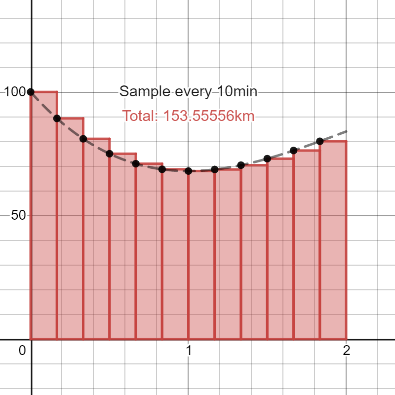
As you can see, the red region is approximately the area under the curve. Thinking back to when you were computing the instantaneous velocity of the falling apple, you figure that your approximation of the total distance covered would get better if you sample more frequently (that is, if you take $\Delta t$ to be ever decreasing), since the velocity will be closer to being constant in smaller time intervals:

(You can experiment with this yourself on Desmos.) Because the approximation keeps approaching the true total distance covered, you realise that the total distance covered is the limit of these approximations as you take $\Delta t\to0$ . To summarise, you find that

$\displaystyle \Delta x_{\mathrm{tot}} = \lim_{\Delta t\to0}\sum_{i=1}^Nv(t_i)\Delta t$

(Working this out for the velocity function in the above picture, you get that the distance travelled is exactly 152km.) Even though you’ve figured out how to solve the problem you gave yourself, there’s still plenty of road left, so you let your mind continue off this tangent.

The integral

If you replace $v(t)$ with an arbitrary function $f(x)$ , it no longer makes as much sense to ask “how far have we travelled,” but the visualisation of the computation still makes sense: the above formula can be used to compute the area under the graph of a function! Suppose I wanted to measure the area under a function $f(x)$ where $a\leq x\leq b$ . Then, just as before, I would sample $f(x)$ at various input values $x_i$ that are all some $\Delta x$ apart, compute the areas of the rectangles of width $\Delta x$ and height $f(x_i)$ , and then sum them up. As long as I assume that my function is nice enough (meaning that my function “looks constant” if I take $\Delta x$ small enough—such a function is called uniformly continuous), then I should get a pretty good approximation for the area, and the approximation should get better and better as I take $\Delta x\to0$ .

To summarise: for a (uniformly continuous) function $f(x)$ , the area of the region under $f(x)$ is given by

$\displaystyle\lim_{\Delta x\to0}\sum_{i=1}^Nf(x_i)\Delta x$

This notation kind of hides $a$ and $b$ (implicitly, $x_1=a$ , and $x_N=b-\Delta x$ ), so to be more explicit, we could abuse notation a little bit and write the above expression instead as

$\displaystyle\lim_{\Delta x\to0}\sum_a^bf(x)\Delta x$

where the summation reads as “sum over values of $x$ that start at $x=a$ , and go up by $\Delta x$ until you reach $x=b$ .” The key, here, is that we are taking $\Delta x\to0$ , which is very similar to what you did to take derivatives of functions. Remember that $\Delta$ is the capital Greek letter “D” and represents “change,” so if you wanted to refer to a “really small change,” suggestive notation would be to use a little $\mathrm d$ . Therefore, if $\Delta x$ is a change in $x$ , then $\mathrm dx$ is a “small” change in $x$ .

Likewise, when $\Delta x\to0$ , the above sum becomes increasingly fine (you sum over the function with increasing resolution), almost making it “smooth.” Since $\Sigma$ is the capital Greek letter “S” (for “sum”), then a smooth sum should be written with a smoother “S” (such as our own English “S”). Adopting this suggestive notation, we get to the more modern notation for the above sum:

$\displaystyle \int_a^bf(x)\mathrm dx = \lim_{\Delta x\to0}\sum_a^bf(x)\Delta x$

This is called the integral of $f(x)$ on the interval $[a,b]$ . As per the above discussion, this computes the area* under $f(x)$ in this interval.

*Technical point. Whenever $f(x)<0$ , the “area under the curve” is negative, so this is more appropriately some kind of “signed” area.

While this does give us a precise way of computing the area under a curve, this is quite tedious to do directly… there’s no way you’d determine how far you travelled by integrating your velocity over the time travelled! If you wanted to determine how far you travelled from time $t=a$ to time $t=b$ , it would be much simpler to take your final position $x(b)$ and take its difference from your initial position $x(a)$ (the mathematical equivalent of just checking your location on the phone).

… So would we able to do a similar thing for other functions? We have two ways of computing how far we travelled: on one hand, we could take the velocity over time and integrate; on the other hand, we can just take the difference of positions (way easier). If they’re both done correctly, then they have to agree, so this gives us a formula

$\displaystyle \int_a^bv(t)\mathrm dt = x(b) - x(a)$

To extend this formula to other functions, you need a way of connecting velocity and position. This is when you remember: velocity is the derivative of position with respect to time!

$\displaystyle v(t) = \frac{\mathrm dx}{\mathrm dt} = \lim_{\Delta t\to0}\frac{\Delta x}{\Delta t}$

This means that if $f(x)$ is the derivative of some other function $F(x)$ (i.e., $\frac{\mathrm dF}{\mathrm dx}=f(x)$ ), then we can view $f(x)$ as a “velocity function” and $F(x)$ as the “position function” and proceed just as you did in the car, and we obtain:

Fundamental Theorem of Calculus. If $\frac{\mathrm dF}{\mathrm dx}=f(x)$ , then

$\displaystyle \int_a^bf(x)\mathrm dx = F(b) - F(a)$

This dramatically simplifies integration from being near impossible to being near impossible only sometimes.

This is all fine and dandy, but then you hear your old physics teacher in your ear: velocity is a vector. Looking out the window, you realise the driver has been taking the scenic route (in the middle of the night)… all of your calculations have been based on just the speed of the car, and so you’ve only figured out how to calculate the total mileage of the vehicle.

So, you redo the entire computation, but this time using a vector-valued function $\vec v(t)=(v_x(t),v_y(t))$ , which at time $t$ gives you the horizontal and vertical components of the velocity of the vehicle. If you divvy up time into small intervals of length $\Delta t$ again (and treating the velocity as constant in each interval), you realise that you’re just doing exactly the same thing as before, but on each component: the total displacement per interval is just a vector whose first component is the horizontal displacement $v_x\cdot\Delta t$ , and whose second component is the vertical displacement $v_y\cdot\Delta t$ . Therefore, you realise that

$\displaystyle \int_a^b\vec v(t)\mathrm dt = \int_a^b\begin{bmatrix} v_x(t) \\ v_y(t)\end{bmatrix}\mathrm dt = \begin{bmatrix} \int_a^bv_x(t)\mathrm dt \\ \int_a^bv_y(t)\mathrm dt\end{bmatrix}$

Let $\vec r(t)=(x(t),y(t))$ be the position (i.e., coordinates) of the vehicle at time $t$ , where $a\leq t\leq b$ . You don’t know what this function is (since you’re still too proud to just check the map), but you remember that its (total) derivative is exactly the velocity vector! Specifically, the horizontal (resp. vertical) component of the velocity is just the derivative of the horizontal (resp. vertical) component of the displacement with respect to time:

$\displaystyle \mathrm D\vec r(t) = \begin{bmatrix} \frac{\mathrm dx}{\mathrm dt} \\[1ex] \frac{\mathrm dy}{\mathrm dt}\end{bmatrix} = \begin{bmatrix} v_x(t) \\ v_y(t) \end{bmatrix} = \vec v(t)$

Therefore, you realise that the Fundamental Theorem of Calculus immediately generalises to higher dimensions:

$\displaystyle \int_a^b\mathrm D\vec r(t)\mathrm dt = \begin{bmatrix} \int_a^bv_x(t)\mathrm dt \\ \int_a^bv_y(t)\mathrm dt\end{bmatrix} \stackrel{\mathrm{FTC}}= \begin{bmatrix} x(b)-x(a) \\ y(b)-y(a) \end{bmatrix} = \vec r(b)-\vec r(a)$

You now lie back, relieved that you’ve accounted for everything. You can finally rest. You look out and watch the moonlit trees as they march over the gentle hills of their domain—

—hills?

You jolt back awake. This isn’t Saskatchewan! You forgot to account for vertical displacement. First, you shrug: if you just use a 3D velocity vector $\vec v(t)=(v_x(t),v_y(t),v_z(t))$ , then the calculation is exactly the same as before, since you just need to integrate each component separately. However, you realise that you don’t really know how to determine your elevation just from sitting in the car… there isn’t really any reference point. You take a drink from your water bottle and collect your thoughts.

Winding paths, up and down hills

That’s when you notice: the surface of the water in your bottle is always level! This gives you an absolute reference point from which you can determine the slope of the car at any point! You collect your data and record that whenever you are in position $(x,y)$ on the map, the vehicle makes a vertical slope of $m(x,y)$ in the direction of the vehicle. Now, you have enough information to calculate your vertical displacement through the trip—it’s just a matter of using the information properly. Recall that the (vertical) slope calculates the ratio

$\displaystyle\text{slope} = \frac{\text{change in height}}{\text{distance travelled}} = \frac{\text{``rise''}}{\text{``run''}}$

We know the slope, and we can calculate how far we travelled. What we want to know is our change in height, so rearrange the formula as

$\text{change in height} = \text{(slope)} \times \text{(distance travelled)}$

In fancier symbols, we can just write this as

$\displaystyle m(x,y) = \frac{\Delta z}{\Delta s} \implies \Delta z = m(x,y)\Delta s$

where $z$ indicates your vertical position (height), and $s$ denotes your position on the road (we originally used $x$ for position, but now that position is 2D we change letters).

Look familiar? This calculation assumes that the slope remains constant throughout the distance $\Delta s$ travelled, but since the roads are hilly, we can only use this as an approximation. By sampling more frequently and taking $\Delta s\to0$ , we can assume that the slope is constant in each interval and then add up these quantities. This is just another integral, so we determine that the overall change in height is just given by the integral

$\displaystyle \int_Cm(x,y)\mathrm ds$

where $C$ denotes the 2D curve describing the entire road trip (i.e., the trace of $\vec r(t)$ for $t\in[a,b]$ ). While this is symbolically nice, we haven’t actually determined how to calculate $\Delta s$ …

Again, to simplify the calculation, pretend that (for a short distance) the car travels in a straight line. If you knew that the car travelled $\Delta x$ and $\Delta y$ in each coordinate (i.e., east and north, respectively), then the Pythagorean Theorem would tell you what the total change of distance is:

$\Delta s^2 = \Delta x^2 + \Delta y^2 \implies \Delta s = \sqrt{\Delta x^2 + \Delta y^2}$

Of course, you don’t actually know the car’s eastward and northward displacements at any position directly: you just know the car’s velocity vector. Fortunately, this is all you need: assuming the eastward (resp. northward) velocity of the car remains constant for a short period of time, then the total eastward (resp. northward) displacement is just given by $\Delta x = v_x\cdot\Delta t$ (resp. $\Delta y=v_y\cdot\Delta t$ ). Plugging this into the above Pythagorean equation, we get

$\Delta s = \sqrt{(v_x\cdot\Delta t)^2 + (v_y\cdot\Delta t)^2} = \sqrt{v_x^2 + v_y^2}\cdot\Delta t$

Notice that $\Delta t$ completely factors out! The expression that’s left is the length (i.e., Euclidean norm) of the velocity vector $\vec v = (v_x, v_y)$ —this is precisely the speed of the car! This shouldn’t be a surprise: we’ve just re-calculated that the distance travelled in that time interval is the speed of the car multiplied by the time interval:

$\Delta s = \|\vec v\|\Delta t \implies \mathrm ds = \|\vec v(t)\|\mathrm dt$

If you integrate this quantity over the entire curve $C$ , you just recover what you did at the very beginning: the total mileage of the car is the integral of the car speed over the duration of the trip. Therefore, “ $\mathrm ds$ ” is often called the length element. We are finally in a position where we can compute the line integral $\int_Cm(x,y)\mathrm ds$ . To give this a convenient overall formula, recall that $\vec v(t) = \mathrm D\vec r(t)$ is the total derivative of the coordinates of the car over time. This gives us the formula

$\displaystyle \int_Cm(x,y)\mathrm ds = \int_a^bm(\vec r(t))\left\|\mathrm D\vec r(t)\right\|\mathrm dt$

If we write $\vec r(t) = (x(t),y(t))$ , then the above formula has an even more explicit form:

$\displaystyle \int_Cm(x,y)\mathrm ds = \int_a^bm(x(t),y(t))\sqrt{\left(\frac{\mathrm dx}{\mathrm dt}\right)^2 + \left(\frac{\mathrm dy}{\mathrm dt}\right)^2}\mathrm dt$

This calculates the total vertical displacement of the car during the road trip, but bells continue to ring in your mind (no, not Christmas bells): if $m(x,y)$ calculates a slope of some kind, then isn’t it a derivative of something? Let $h(x,y)$ denote the actual elevation of the land at any point $(x,y)$ , then indeed $m(x,y)$ is the directional derivative of $h(x,y)$ in the direction of the car’s velocity at the point $(x,y)$ .

Remembering back to computing derivatives of higher-dimensional functions, you remember that directional derivatives can be computed using the gradient $\vec F := \nabla h$ : the directional derivative of $h(x,y)$ in the direction of the unit vector $\vec u$ is given by

$\nabla_{\vec u}h(x,y) = \vec F(x,y)\cdot\vec u$

It’s important that $\vec u$ is a unit vector in this calculation. If we are given a general (nonzero) vector $\vec v$ , then the unit vector describing its direction can be calculated by normalising it as $\vec u = \frac{\vec v}{\|\vec v\|}$ . Therefore, the slope function $m(x,y)$ can be written in terms of $h(x,y)$ as

$\displaystyle m(x,y) = \vec F(x,y)\cdot\frac{\vec v}{\|\vec v\|}$

Interesting: if you recall, $\mathrm ds=\|\vec v\|\mathrm dt$ . This means that integrating the above quantity with respect to the length element causes the norms $\|\vec v\|$ to cancel out! Therefore, plugging this in (and remembering that $\vec v = \mathrm D\vec r$ ), we get that

$\displaystyle \int_Cm(x,y)\mathrm ds = \int_a^b\vec F(\vec r(t))\cdot\frac{\mathrm D\vec r(t)}{\|\mathrm D\vec r(t)\|}\|\mathrm D\vec r(t)\|\mathrm dt = \int_a^b\vec F(\vec r(t))\cdot\mathrm D\vec r(t)\mathrm dt$

If we write out the components of $\vec F$ (which may be called a vector field) as $\vec F = (P, Q)$ , then the above dot product may be expanded to give an even more explicit form

$\displaystyle \int_a^b\vec F(\vec r(t))\cdot\mathrm D\vec r(t)\mathrm dt = \int_a^b\left[P(x(t),y(t))\frac{\mathrm dx}{\mathrm dt} + Q(x(t),y(t))\frac{\mathrm dy}{\mathrm dt}\right]\mathrm dt$

By “cancelling out” the $\mathrm dt$ terms, this gives us some of the more lazy notations for the same line integrals:

$\displaystyle \int_C\vec F\cdot\mathrm d\vec r := \int_CP\mathrm dx + Q\mathrm dy := \int_a^b\vec F(\vec r(t))\cdot\mathrm D\vec r(t)\mathrm dt$

but I digress. In any case, because the total vertical displacement can be computed most simply as the difference $h(\vec r(b)) - h(\vec r(a))$ , your derivation above can be summarised as:

Fundamental Theorem of Calculus for line integrals. If $\vec F = \nabla h$ for some ( $n$ -variate) function $h$ , and $C$ is a curve that is parametrised by some $\vec r:[a,b]\to\mathbb{R}^n$ , then

$\displaystyle \int_C\vec F\cdot\mathrm d\vec r = h(\vec r(b)) - h(\vec r(a))$

Victory! Even you have to admit you’ve done an impressive amount of impromptu mathematics thus far. Surely you must be coming close to your travel destination by now.

Don’t call your driver Shirley: to your surprise, there is still quite a ways to go. “Unbelievable,” you think. “With how much time has passed, we must have travelled halfway around the world by now!” Your exasperation comes to an abrupt halt: around the world? Egad; you haven’t accounted for the curvature of the Earth.

Going great lengths on Earth

Fortunately, you already have the groundwork necessary for talking about calculus on Earth: smooth manifolds. For simplicity, you model the Earth with the standard 2-sphere

$\mathbb{S}^2 := \{(x,y,z)\in\mathbb{R}^3 \mid x^2+y^2+z^2=1\}$

Of course, this is just a model. You know there are mountains and valleys on Earth, but you’ll deal with that issue later; the more pressing issue is how to make sure that you track distances on the sphere appropriately. Given two points on a 2-sphere, how do you determine their distance?

At face value, you could just embed the sphere into three-dimensional space and then measure the points’ Euclidean distance, but this measures the length of the straight line between the points. Given what you’re trying to do (measure mileage of the car on Earth), this isn’t a particularly useful notion of distance. A more relevant measurement is the length of arcs on Earth between the points, rather than straight lines. If you wanted to get the distance between points from the perspective of someone living on the 2-sphere, you could then just measure the smallest such length (which in this case would be the length of the geodesic connecting the two points).

Again, you could just embed the 2-sphere into three-dimensional (Euclidean) space and then measure the length of any arc through this embedding, but this is more of an extrinsic definition of arclength and could very well depend on how you embed the 2-sphere into Euclidean space, so it’s not an entirely satisfactory answer. Is there a way to measure these arclengths without an embedding?

To help answer this question, you revisit your formula for arclength in Euclidean space. If $C$ is a curve parametrised by a (smooth) function $\vec r:[a,b]\to\mathbb{R}^n$ , then the length of $C$ was given by the integral

$\displaystyle \mathrm{len}(C) = \int_C\mathrm ds = \int_a^b\|\mathrm D\vec r(t)\|\mathrm dt$

In English, the length of the curve is just determined as follows: have a particle travel along the curve and track its speed over time (this is $\|\mathrm D\vec r(t)\|$ ), then add this over the entire duration of the travel. On a manifold $M$ , an arc is replaced by the trace of a function $\gamma:[a,b]\to M$ , so what would the analogue in this setting look like?

If you picture $\gamma$ as parametrising the path of a particle on the manifold, then you recall that the velocity of the particle at a given time $t$ is precisely a tangent vector of $M$ at the point $\gamma(t)\in M$ ; that is, an element of $T_{\gamma(t)}M$ . The speed of the particle would then be the length of this tangent vector.

Since $T_pM$ is a (real) vector space of dimension equal to the dimension of the manifold $M$ (say of dimension $n$ ), it might be tempting to take the Euclidean length of these tangent vectors. However, there’s a small issue: the Euclidean metric on $\mathbb{R}^n$ is determined by the dot product, and the dot product is computed using the standard basis of $\mathbb{R}^n$ . Although $T_pM$ can be given a basis for every point $p\in M$ , there isn’t actually any canonical way of doing it in general. Usually, the basis is given by the partial derivatives $\left.\frac\partial{\partial x_1}\right|_p,\dots,\left.\frac\partial{\partial x_n}\right|_p$ , but this basis depends on the choice of coordinate chart $x_1,\dots,x_n$ at the point.

The point is that a canonical basis can’t be generally chosen for a manifold in a consistent way (manifolds which admit a basis of its tangent spaces that vary smoothly are called parallelisable). Therefore, to be able to measure arclengths, you need to endow the manifold with additional structure that gives a metric on tangent spaces in a “nice” way. This is done by endowing the manifold $M$ with a function $g_p:T_pM\times T_pM\to\mathbb{R}$ at every point $p\in M$ that looks like the dot product, and changes smoothly as you change $p$ . A manifold equipped with such a structure is called a Riemannian manifold. The functions $g_p$ form the so-called Riemannian metric.

Formal definition (skippable). A Riemannian $n$ -manifold is a pair $(M,g)$ where $M$ is a smooth $n$ -manifold, and $g$ assigns to every point $p\in M$ an inner product $g_p:T_pM\times T_pM\to\mathbb{R}$ smoothly in the sense that if $x_1,\dots,x_n$ are local coordinates on an open set $U\subseteq M$ , then for all $1\leq i,j\leq n$ ,

$U\to\mathbb{R}, \qquad p\mapsto g_{i,j}|_p := g_p\left(\left.\frac\partial{\partial x_i}\right|_p,\left.\frac\partial{\partial x_j}\right|_p\right)$

is a smooth function of $p$ (after identifying $U\cong\mathbb{R}^n$ via the local coordinates). We may also denote the Riemannian metric by $\mathrm ds^2$ .

Given a Riemannian metric, you can then define norms on the tangent spaces in the same way as you would with the dot product in Euclidean space: the norm of a tangent vector $v\in T_pM$ is just $|v|_p := \sqrt{g_p(v,v)}$ . Now, if $\gamma:[a,b]\to M$ parametrises some curve $C$ in our Riemannian manifold, then its length is the (ordinary) integral

$\displaystyle \mathrm{len}(C) := \int_C\mathrm ds := \int_a^b\left|\mathrm d\gamma_t\right|_{\gamma(t)}\mathrm dt$

Once you find an appropriate Riemannian metric on the 2-sphere, this would handle the total distance travelled by the car given that the Earth is perfectly spherical. This is a similar situation as when you forgot to account for hills. To account for mountains and valleys, you need to introduce a height function $h:M\to\mathbb{R}$ which gives you the elevation $h(p)$ at any point $p\in M$ . A suitable integral of this function should then compute the total vertical displacement.

By the same reasoning as in the Euclidean setting, you want to integrate the directional derivative of $h$ along the curve $\gamma$ . In this setting, the analogue of the gradient of $h$ is just its derivative $\mathrm dh:TM\to T\mathbb{R}$ . At any point $p\in M$ , this gives a linear functional $\mathrm dh_p:T_pM\to T_{h(p)}\mathbb{R}\cong\mathbb{R}$ ; that is, an element of the dual space of $T_pM$ .

Recall that the derivative of a function of manifolds is given by the Jacobian matrix when written in terms of (partial derivatives of) local coordinates. In particular, $\mathrm dh$ locally looks like the gradient of $h$ at any point, and the composite $\mathrm dh_p(v)\in\mathbb{R}$ for a (unit) tangent vector $v\in T_pM$ is therefore locally the same as the directional derivative of $h$ in the direction $v$ . Since directional derivatives are a local concept, this makes the analogy “solid.” In particular, integrating the directional derivatives over the arc recovers the same old integral computation as before: if $C\subseteq M$ is a curve parametrised by the function $\gamma:[a,b]\to M$ , then

$\displaystyle \int_C\mathrm dh = \int_{p\in C}\left[\mathrm dh\left(\frac{\mathrm d\gamma}{|\mathrm d\gamma|_p}\right)\right]\mathrm ds = \int_a^b\left[\mathrm dh\left(\frac{\mathrm d\gamma_t}{|\mathrm d\gamma_t|_{\gamma(t)}}\right)|\mathrm d\gamma_t|_{\gamma(t)}\right]\mathrm dt = \int_a^b\big[\mathrm dh(\mathrm d\gamma_t)\big]\mathrm dt$

In particular, the Riemann metric cancels out! Therefore, although we need a Riemannian metric to integrate with respect to arclength, Riemannian structure is unnecessary for integrating… things that look like $\mathrm dh$ .

What exactly are such things? In the Euclidean setting, we treated the gradient $\nabla h$ as a sort of vector field, but the fact that $\mathrm dh_p$ is a map $T_pM\to\mathbb{R}$ shows that this perspective is not quite perfect. In particular, since we only used the gradient as a means to compute directional derivatives (via the dot product), it seems more appropriate to view the gradient as a covector field; that is, a smoothly varying family of linear functionals on the tangent space. We could afford oversimplifying the gradient as a vector field because finite-dimensional vector spaces have the same dimension as their dual space, but now it hampers our understanding of the theory.

But why would we prefer linear functionals on the tangent space more than actual tangent vectors when integrating? It may not entirely make sense why these are suitable: an integral is fundamentally a formalisation of an “infinite sum of infinitesimal quantities,” so what do linear functionals have to do with infinitesimals? To answer this, let’s try to be more precise about what “infinitesimal changes” should be on a manifold.

There is no one way to go about this, but first we should declare what we intend to measure infinitesimal changes of. This is fairly simple: for our purposes (integration), we’re mostly interested in infinitesimal changes of functions. Note that we’re talking about the infinitesimal changes themselves, rather than the infinitesimal rates of changes (we have already figured out the latter up to the generality of manifolds; in symbols, for a function $f(x)$ , we are now more interested in $\mathrm df$ rather than $\frac{\mathrm df}{\mathrm dx}$ ). Therefore, for the sake of integrating, we want to define a space

$T^*_pM := \{\text{infinitesimal changes of functions defined around the point } p\}$

In particular, we’re less concerned with specific functions, and are more focused on their infinitesimal changes. Therefore, we should consider two functions defined around a point $p$ to be “the same” as elements of $T^*_pM$ if their infinitesimal changes are the same at the point $p$ in some sense. Since we only care about how functions behave in the immediate vicinity of the point $p$ , a step towards this end would be to consider two functions to be “the same” if they are equal in a sufficiently small neighbourhood of the point $p$ . This defines the space $\mathcal O_{M,p}$ of germs of functions defined near the point $p\in M$ .

Germs of functions almost extract the infinitesimal information of a function at a point—they extract the local information of a function. However, since we’re more interested infinitesimal changes of a function, it doesn’t even matter to us what the function is equal to at $p$ : the infinitesimal changes of a function $f(x)$ ought to be the same as the infinitesimal changes of the translated function $f(x)+k$ , where $k\in\mathbb{R}$ is some constant. We can go about ignoring the effect of this translation in two (equivalent) ways:

(quotient) we can declare that two functions $f,g$ are “the same” if their difference $f-g$ is equal to a constant function
(normalise) we can just restrict our attention to just those functions $f\in\mathcal O_{M,p}$ where $f(p)=0$

Choose the latter for simplicity and define

$\mathfrak m_p := \{f\in\mathcal O_{M,p} \mid f(p) = 0\}$

Note that for any function $g(x)\in\mathcal O_{M,p}$ , we can normalise it to get an element of $\mathfrak m_p$ by replacing it with the difference $g(x)-g(p)$ . This is how to show that the two approaches mentioned above are equivalent.

Remark (skippable). In fancy jargon, a ring of germs at a point is precisely a stalk of the sheaf of functions on the manifold: if $\mathcal O_M(U) := C^\infty(U,\mathbb{R})$ is the ring of smooth functions on an open subset $U\subseteq M$ , then

$\displaystyle \mathcal O_{M,p} = \varinjlim_{U\ni p}\mathcal O_M(U)$

The reason we denote the subcollection of (germs of) functions that vanish at $p$ by $\mathfrak m_p$ is because it is the unique maximal ideal in $\mathcal O_{M,p}$ .

The space $\mathfrak m_p$ encodes the “local perturbations” of a function, but unfortunately does not encode the infinitesimal perturbations. To see evidence of this, consider the functions below:

Functions with arguably identical infinitesimal changes but different germs at $p=0$ _[Desmos]

Functions with arguably identical infinitesimal changes but different germs at $p=0$ _[Desmos]

No matter how closely you zoom into the origin, these functions are never equal away from zero, meaning that their germs are different in $\mathfrak m_0\subset\mathcal O_{\mathbb{R},0}$ . However, it seems like their infinitesimal perturbations at zero should be equal. The problem is most obvious when you consider the function $f(x)=x^2$ . At the origin, how would you describe its infinitesimal perturbation? There should be none: the function is essentially flat at zero. Therefore, $f$ should be trivial in $T_0^*\mathbb{R}$ .

You might notice at this point that although we’ve made a distinction between infinitesimal changes and derivatives, we’re essentially declaring that two functions have the same infinitesimal changes if their derivatives are the same! Therefore, we define $T_p^*M$ to be the space $\mathfrak m_p$ , but we think of two functions $f,g\in\mathfrak m_p$ as “the same” if $\mathrm df_0=\mathrm dg_0$ . This makes $T_p^*M$ really look like the space of infinitesimal changes of functions at $p\in M$ .

So what does this have to do with linear functionals on the tangent space? Well, it turns out that there is a natural identification of $T_p^*M$ with the dual space $(T_pM)^\vee$ of the tangent space!

Indeed, the derivative defines a linear map $\mathrm d : T_p^*M\to(T_pM)^\vee$ by sending a function $f\in T_p^*M$ to its derivative $\mathrm df:T_pM\to T_p\mathbb{R}\cong\mathbb{R}$ . Since we identify functions in $T_p^*M$ if they have the same derivative, this linear map is injective. On the other hand, fix a local coordinate system $x_1,\dots,x_n$ around $p$ . Each coordinate is a local function, where $x_i$ takes in a point near $p$ and spits out its $i$ th coordinate in this local coordinate system. This gives us $n$ functions $x_1,\dots,x_n$ in $T_p^*M$ , and it turns out that they are linearly independent! Indeed, this is best seen by checking their derivatives: now that we have local coordinates, derivatives in these coordinates look like gradients, and so in these coordinates,

$\mathrm (dx_i)_p \doteq e_i^\top = \begin{bmatrix} 0 & \dots & 1 & \dots & 0 \end{bmatrix}$

showing that their derivatives are linearly independent in $(T_pM)^\vee$ . Since this means we have an injective linear transformation from a space $T_p^*M$ of dimension $\geq n$ and a space $(T_pM)^\vee$ of dimension $n$ , it follows that this transformation must be a linear isomorphism: there is a natural correspondence between infinitesimal changes of functions and linear functionals on the tangent space. What’s more, our above argument also proves that any local coordinate system near $p$ gives us a basis of $T_p^*M=(T_pM)^\vee$ given by the differentials $(\mathrm dx_1)_p,\dots,(\mathrm dx_n)_p$ , and this basis is dual to the basis $\left.\frac\partial{\partial x_1}\right|_p,\dots,\left.\frac\partial{\partial x_n}\right|_p$ of $T_pM$ in the sense that

$\displaystyle \mathrm dx_i\left(\left.\frac\partial{\partial x_j}\right|_p\right) = \left.\frac{\partial x_i}{\partial x_j}\right|_p = \delta_{i,j} = \begin{cases} 1, & \text{if } i=j \\ 0, & \text{if } i\neq j \end{cases}$

Summary/Definition. For a smooth $n$ -manifold $M$ and a point $p\in M$ , define the cotangent space at $p$ to be the dual space $T^*_pM := (T_pM)^\vee$ of the tangent space at $p$ . Moreover, if $x_1,\dots,x_n$ is a local coordinate system near $p$ , then denote the dual basis in $T^*_pM$ corresponding to $\left.\frac\partial{\partial x_1}\right|_p,\dots,\left.\frac\partial{\partial x_n}\right|_p\in T_pM$ by $\mathrm dx_1,\dots,\mathrm dx_n$ .

Remark (skippable). The above work is just the first isomorphism theorem spelled out: using the local coordinate functions, we proved that the derivative map $\mathrm d:\mathfrak m_p\to(T_pM)^\vee$ is surjective, and therefore induces an isomorphism $\frac{\mathfrak m_p}{\mathrm{ker}(\mathrm d)}\cong(T_pM)^\vee$ . On the other hand, in the discussion, we define the space $T^*_pM$ as precisely this quotient.

Taking one more step, we get a more useful definition of the cotangent space. Given two smooth functions that vanish at zero, their product must have a trivial derivative by the product rule. Therefore, we get an inclusion $\mathfrak m_p^2\hookrightarrow\mathrm{ker}(\mathrm d)$ (where $\mathfrak m_p^2$ is the ideal generated by products of elements of $\mathfrak m_p$ ). This inclusion is in fact an isomorphism (a high-powered reason is by looking at Taylor expansions in local coordinates), meaning $\mathfrak m_p^2=\mathrm{ker}(\mathrm d)$ . This gives another equivalent definition of the cotangent space as the quotient $T_p^*M := \frac{\mathfrak m_p}{\mathfrak m_p^2}$ , which comes in handy for instance in algebraic geometry.

Using this newfound notation, we get a formalisation of the differential of a function discussed back when you studied derivatives. If we fix a local coordinate system $x_1,\dots,x_n$ around $p$ , then the derivative of a function $f$ looks like a gradient in the induced basis on the tangent space since $\mathrm df\left(\left.\frac\partial{\partial x_i}\right|_p\right) = \left.\frac{\partial f}{\partial x_i}\right|_p$ . Therefore, using the induced basis on the cotangent space, we recover the familiar formula

$\displaystyle \mathrm df_p = \left.\frac{\partial f}{\partial x_1}\right|_p\mathrm dx_1 + \dots + \left.\frac{\partial f}{\partial x_n}\right|_p\mathrm dx_p$

In particular, if we smoothly vary our choice of $p$ (as well as the associated local coordinates), the coefficients of each $\mathrm dx_i$ vary smoothly as well. This gives us a better idea of what can be integrated over a curve in a manifold (i.e., what a covector field ought to be): a covector field $\omega$ on our manifold assigns to every point $p\in M$ an element $\omega_p\in T_p^*M$ in a way that “varies smoothly” with $p$ . In local coordinates, such a covector field thus takes the form $\omega = f_1(p)\mathrm dx_1 + \dots + f_n(p)\mathrm dx_n$ , where $f_1,\dots,f_n$ are smooth (local) functions. Therefore, such covector fields are also called differential 1-forms, and we denote the space of all differential 1-forms on $M$ by $\Omega^1(M)$ .

Remark. We make precise the idea of making choice of cotangent vectors “smooth” by constructing the cotangent bundle $T^*M$ on $M$ , which is done in a similar way to the tangent bundle $TM$ . In particular, the cotangent bundle is a smooth manifold with a projection map $\pi:T^*M\to M$ (sending a cotangent vector in $T^*_pM$ to $p$ ). With the structure of a vector bundle, a differential 1-form is precisely a smooth section of the cotangent bundle, meaning that it is a smooth map $\omega:M\to T^*M$ such that $\pi\circ\omega=\mathrm{id}$ ; that is, $\omega_p\in T_p^*M$ for every $p\in M$ .

Analogously, a vector field on $M$ is just a section of the tangent bundle; that is, a function $F:M\to TM$ such that $F(p)\in T_pM$ for every $p\in M$ . In the presence of a Riemannian metric $g$ , we get a canonical identification of vector fields with differential 1-forms by identifying the vector field $F$ with the form $\omega\in\Omega^1(M)$ given by $\omega_p := g(F(p),-)$ .

Suppose we have a Riemannian metric $\mathrm ds^2$ on our manifold. Then, we can integrate a differential form $\omega$ in the same way that we integrated the derivative of a function as before. Intuitively, given a unit tangent vector $u\in T_pM$ , the value of $\omega_p(u)$ represents the infinitesimal change $\omega_p$ in the direction $u$ . Therefore, to accumulate these directional infinitesimal changes along a curve $C$ parametrised by some function $\gamma:[a,b]\to M$ , we proceed as before:

$\displaystyle \int_C\omega := \int_{p\in C}\left[\omega\left(\frac{\mathrm d\gamma}{|\mathrm d\gamma|_p}\right)\right]\mathrm ds = \int_a^b\left[\omega\left(\frac{\mathrm d\gamma_t}{|\mathrm d\gamma_t|_{\gamma(t)}}\right)|\mathrm d\gamma_t|_{\gamma(t)}\right]\mathrm dt = \int_a^b\big[\omega(\mathrm d\gamma_t)\big]\mathrm dt$

Once again, the final formula is left independent of the metric! Therefore, we can define the integral of a differential 1-form over curves on arbitrary* manifolds this way.

*Technical remark. In general, integration of forms requires first fixing an orientation of the manifold. This is implicit in the above formula, because it assumes that the curve $C$ is oriented (for a curve, this means it flows in one direction), and that the parametrisation $\gamma:[a,b]\to M$ preserves this orientation. This is important because if you trace the curve in the other direction, then the resulting integral will be the negative of the original, just like how $\int_a^bf(x)\mathrm dx = -\int_b^af(x)\mathrm dx$ . Once we’re in this situation, the integral $\int_C\omega$ is given by the above formula. It may also be worth noting that every smooth manifold can be given some Riemannian metric.

It may have been so long that the original goal has been forgotten, but remember: all this was to understand how to integrate the derivative of a height function $h:\mathbb{S}^2\to\mathbb{R}$ on the 2-sphere, and from entirely analogous analysis as in the Euclidean setting, this integral computes the total vertical (i.e., “outward” in the direction $h$ measures) displacement accrued along the path travelled. In symbols:

Generalised Stokes’ Theorem in one dimension. If $M$ is a smooth manifold and $C\subseteq M$ is an orientable curve that is parametrised by a smooth (orientation-preserving) function $\gamma:[a,b]\to M$ . Then for all smooth functions $f:M\to\mathbb{R}$ , we have

$\displaystyle \int_C\mathrm df = f(b) - f(a)$

which further generalises the “fundamental theorems” of calculus established much earlier.

This would have been a good place to end things, but we haven’t yet established a Riemannian metric on the 2-sphere, so we can’t yet compute the actual arclength of the journey $C$ . Therefore, let’s end this by saying a few more words about this.

Measuring great lengths on Earth

First, the notation $\mathrm ds^2$ for the Riemannian metric suggests that—just like in the Euclidean setting when computing arclengths—the metric is somehow a product of differentials. While not precisely true, there is an element of truth to it. Recall that a Riemannian metric is a smoothly-varying assignment of inner products $g_p$ on $T_pM$ . Inner products are, in particular, bilinear, and so can be instead described as a linear map from the tensor product $g_p:T_pM\otimes T_pM\to\mathbb{R}$ . This means that $g_p$ is a particular element of the dual space $(T_pM\otimes T_pM)^\vee$ . Since tangent spaces are finite-dimensional, we can equivalently identify $g_p$ with a particular element of $T^*_pM\otimes T^*_pM$ in a canonical way.

Let’s be more explicit about this. If we fix a local coordinate system $x_1,\dots,x_n$ , then the Riemannian metric is locally determined by the coefficients $g_{i,j}|_p := g_p\left(\left.\frac\partial{\partial x_i}\right|_p,\left.\frac\partial{\partial x_j}\right|_p\right)\in\mathbb{R}$ for the $p\in M$ in this local coordinate system. With these coefficients, we may write the Riemannian metric in terms of the local coordinates as a sum

$\displaystyle \mathrm ds^2 \doteq \sum_{i,j=1}^ng_{i,j}\ \mathrm dx_i\otimes\mathrm dx_j$

where $g_{i,j}$ is a smooth function of $p$ , and (to be extremely explicit) the tensor product $\mathrm dx_i\otimes \mathrm dx_j$ is a bilinear form completely determined by the rule

$\displaystyle \mathrm dx_i\otimes\mathrm dx_j\left(\frac\partial{\partial x_k}, \frac\partial{\partial x_l}\right) = \delta_{i,k}\delta_{j,l} = \begin{cases} 1, & i=k; j=l \\ 0, & \text{otherwise} \end{cases}$

For instance, the usual Euclidean metric on $\mathbb{R}^2$ is defined by $\mathrm ds^2 = \mathrm dx\otimes\mathrm dx + \mathrm dy\otimes\mathrm dy$ , which (for brevity) may also be written in the familiar form $\mathrm ds^2 = \mathrm dx^2 + \mathrm dy^2$ .

Remark (skippable). This perspective also allows us to be more precise about how a Riemannian metric varies smoothly: the Riemannian metric must in particular be a smooth section of the tensor product bundle $T^*M\otimes T^*M$ . For this reason, the Riemannian metric is also often called a metric tensor. More generally, a tensor field of type $(p,q)$ is a smooth section of the vector bundle $(TM)^{\otimes p}\otimes (T^*M)^{\otimes q}$ , showing that the Riemannian metric is a tensor of type $(0,2)$ .

Now for the sake of completeness, let’s derive a metric tensor $g$ on the 2-sphere. We do so by parametrising the 2-sphere using usual polar and azimuthal angles (i.e., spherical coordinates)

$\displaystyle \begin{bmatrix} x_1 \\ x_2 \\ x_3 \end{bmatrix} = \begin{bmatrix} R\cos\theta_1 \\ R\sin\theta_1\cos\theta_2 \\ R\sin\theta_1\sin\theta_2 \end{bmatrix} =: \varphi(\theta_1,\theta_2)$

where $R$ is a fixed radius (meant to be the radius of the Earth, in your situation). This makes $(\theta_1,\theta_2)$ the coordinate system for the sphere via the mapping $\varphi:\mathbb{S}^2\to\mathbb{R}^3$ . We then define the metric on the sphere by pulling back the Euclidean metric along $S$ .

In general, pulling back a metric $g$ on $M$ along some $\varphi:N\to M$ gives a metric $\varphi^*g$ on $N$ such that for a local coordinate system $y_1,\dots,y_m$ of $N$ we have $\varphi^*g\left(\frac\partial{\partial y_i},\frac\partial{\partial y_j}\right) = g\left(\frac\partial{\partial y_i}\circ\mathrm d\varphi,\frac\partial{\partial y_j}\circ\mathrm d\varphi\right)$ . Therefore, the components of the pullback metric are determined by

$\displaystyle (\varphi^*g)_{i,j} = \sum_{k,l}g_{k,l}\frac{\partial x_k}{\partial y_i}\frac{\partial x_l}{\partial y_j}$

where $\varphi(y_1,\dots,y_m) = (x_1,\dots,x_n)$ in a local coordinate system of $M$ .

In our case, the off-diagonal components of the Euclidean metric tensor are zero, so the above expressio simplifies to $g_{i,j} = \sum_k\frac{\partial x_k}{\partial\theta_i}\frac{\partial x_k}{\partial\theta_j}$ . In particular:

$g_{1,1} = \left(\frac{\partial(R\cos\theta_1)}{\partial\theta_1}\right)^2 + \left(\frac{\partial(R\sin\theta_1\cos\theta_2)}{\partial\theta_1}\right)^2 + \left(\frac{\partial(R\sin\theta_1\sin\theta_2)}{\partial\theta_1}\right)^2 = R^2$
$g_{1,2} = \frac{\partial(R\sin\theta_1\cos\theta_2)}{\partial\theta_1}\frac{\partial(R\sin\theta_1\cos\theta_2)}{\partial\theta_2} + \frac{\partial(R\sin\theta_1\sin\theta_2)}{\partial\theta_1}\frac{\partial(R\sin\theta_1\sin\theta_2)}{\partial\theta_2} = 0$
similarly $g_{2,1}=0$
$g_{2,2} = \left(\frac{\partial(R\sin\theta_1\cos\theta_2)}{\partial\theta_2}\right)^2 + \left(\frac{\partial(R\sin\theta_1\sin\theta_2)}{\partial\theta_2}\right)^2 = R^2\sin^2\theta_1$

Therefore, the Riemannian metric on the 2-sphere we get as a result is

$\mathrm ds^2 = R^2\Big[\mathrm d\theta_1^2 + \sin^2\theta_1\mathrm d\theta_2^2\Big]$

At last, you feel the car come to a stop, and your mates all cheer. You’ve arrived at your destination, and right on time for you to wrap up this train of thought! While not the most impactful way to finish the thought, you don’t mind because you know nobody else will follow your thoughts far enough to notice.